Healthcare Pricing and Competition
Table of contents
- Competition in Theory
- Competition in Practice
Competition in Theory
Fixed Prices
- Demand: \(q_{j}=s_{j}(z_{j}) \times D(\bar{p})\)
- Costs: \(c_{j}=c(q_{j},z_{j}) + F\)
- Profits: \(\pi_{j} = \bar{p}q_{j} - c_{j}\)
Hospitals choose quality such that: \[\frac{\partial \pi_{j}}{\partial z_{j}} = \left(\bar{p} - \frac{\partial c_{j}}{\partial q_{j}} \right)\left(\frac{\partial s_{j}}{\partial z_{j}}D + s_{j}\frac{\partial D}{\partial z_{j}} \right) - \frac{\partial c_{j}}{\partial z_{j}}=0\]
Fixed Prices
- Increase in competition will tend to increase quality
- Negative welfare effects if \(\frac{\partial D}{\partial z_{j}}\) is sufficiently small and fixed costs are large
Fixed Prices
Alternative expression for quality: \[z_{j} = \left(\bar{p} - c_{q} \right) \left(\eta_{s} + \eta_{D} \right) \frac{D s_{j}}{c_{z}}\]
- Quality increasing in \(\bar{p}\)
- Quality increasing in share and demand elasticities
- Quality increase in overall market share and market demand
- Quality decreasing in marginal cost
Market Prices
Profit given by \(\pi = q(p,z) \times (p-c-d\times z) - F,\) which yields
\[\begin{align*} p &= \frac{\epsilon_{p}}{\epsilon_{p}-1} (c+dz) \\ z &= \frac{\epsilon_{z}}{\epsilon_{z}+1} \frac{p-c}{d} \end{align*}\]
Market Prices
Rewrite in terms of elasticities:
\[\begin{align*} \epsilon_{p} &= \frac{p}{p-c-dz} \\ \epsilon_{z} &= \frac{dz}{p - c - dz} \end{align*}\]
Taking the ratio and solving for \(z\) yields, \[z = \frac{p}{d}\times \frac{\epsilon_{z}}{\epsilon_{p}}.\]
Market Prices
\[z = \frac{p}{d}\times \frac{\epsilon_{z}}{\epsilon_{p}}\]
Dorfman-Steiner condition:
- Quality increases if the quality elasticity increases or if price increases
- Quality increases if the price elasticity decreases or the marginal cost of quality decreases
Prediction for competition: Hospitals will compete on whatever matters most to patients.
Bargaining
Basic Bargaining Model
Gowrisankaran, Nevo, and Town extend the Nash bargaining framework to consider a hospital-insurer negotiation. They propose a two-stage bargaining process:
- Hospitals and insurers negotiate over the terms of their agreement (network inclusion and prices)
- Individuals receive “health draws” which dictate their healthcare needs
Bargaining occurs over a base price, not specific to each procedure
Basic Bargaining Model
- Total expected cost to the insurer, \(TC_{m}(N_{m},\vec{p}_{m})\)
- Willingness to pay to have access to hospital, \(W_{m}(N_{m},\vec{p}_{m})\)
- Total payoff for the MCO is \[V_{m}(N_{m},\vec{p}_{m}) = \tau W_{m}(N_{m},\vec{p}_{m}) - TC_{m}(N_{m},\vec{p}_{m}),\] where \(\tau\) is the relative weight placed on employee/patient welfare
- Net value that MCO \(m\) receives from including hospital \(j\) in its network is then \(V_{m}(N_{m},\vec{p}_{m})-V_{m}(N_{m,-j},\vec{p}_{m})\).
Basic Bargaining Model
In the case of a single hospital system, and denoting hospital \(j\)’s marginal cost for services provided to patients in MCO \(m\) is given by \(mc_{mj}\), the overall profit for hospital \(j\) for a given set of MCO contracts (denoted \(M_{s}\)), is \[\pi_{j}\left(M_{s},\{\vec{p}_{m}\}_{m\in M_{s}} \right)=\sum_{m\in M_{s}} q_{mj}(N_{m},\vec{p}_{m}) \left[p_{mj} - mc_{mj} \right].\]
Basic Bargaining Model
The authors then derive the Nash bargaining solution as the choice of prices maximizing the exponentiated product of the net value from agreement:
\[\begin{align*} NB^{m,j} \left(p_{mj} | \vec{p}_{m,-j}\right) &= \left(q_{mj}(N_{m},\vec{p}_{m}) \left[p_{mj} - mc_{mj} \right]\right)^{b_{j(m)}} \\ & \times \left(V_{m}(N_{m},\vec{p}_{m})-V_{m}(N_{m,-j},\vec{p}_{m})\right)^{b_{m(j)}}, \end{align*}\]
where \(b_{j(m)}\) is the bargaining weight of hospital \(j\) when facing MCO \(m\), \(b_{m(j)}\) is the bargaining weight of MCO \(m\) when facing hospital \(j\), and \(\vec{p}_{m,-j}\) is the vector of prices for MCO \(m\) and hospitals other than \(j\). We can normalize bargaining weight such that \(b_{j(m)} + b_{m(j)} = 1\).
Basic Bargaining Model
Taking the natural log, the resulting first order condition yields:
\[\begin{align*} \frac{\partial \ln (NB^{m,s})}{\partial p_{mj}} =& b_{s(m)} \frac{q_{mj} + \frac{\partial q_{mj}}{\partial p_{mj}} \left[p_{mj}-mc_{mj}\right]}{q_{mj}\left[p_{mj}-mc_{mj}\right]} \\ & + b_{m(j)} \frac{\frac{\partial V_{m}}{\partial p_{mj}}}{V_{m}(N_{m},\vec{p}_{m})-V_{m}(N_{m,-j},\vec{p}_{m})} = 0 \end{align*}\]
Basic Bargaining Model
Simplifying and rewriting, we get: \[p_{mj} - mc_{mj} = -q_{mj} \left(\frac{\partial q_{mj}}{\partial p_{mj}} + q_{mj} \times \frac{b_{m(j)}}{b_{j(m)}} \times \frac{\frac{\partial V_{m}}{\partial p_{mj}}}{\triangle V_{m}} \right)^{-1}\]
- \(\triangle V_{m}\) is positive by construction
- Can show that \(\frac{\partial V_{m}}{\partial p_{mj}}<0\) under most conditions
Bargaining tends to increase the “effective” price sensitivity and reduce hospital margins relative to standard pricing conditions (but not always)
Basic Bargaining Model
- Price response to other changes depends largely on \(\frac{\partial V_{m}}{\partial p_{mj}}\)
- Can be expressed as: \[-q_{mj}-\alpha \sum_{i}\sum_{d}\gamma_{id}c_{id}(1-c_{id}) \left(\sum_{k\in N_{m}} p_{mk}s_{ikd} - p_{mj}\right),\] where \(\gamma_{id}\) includes several terms including disease weights and probability of disease.
Basic Bargaining Model
\[-q_{mj}-\alpha \sum_{i}\sum_{d}\gamma_{id}c_{id}(1-c_{id}) \left(\sum_{k\in N_{m}} p_{mk}s_{ikd} - p_{mj}\right),\]
- \(c_{id}\) denotes the coinsurance rate
- final term is the difference between hospital \(j\)’s price and the weighted average price of all other hospitals (weighted by their market share)
- \(c_{id}\times (1-c_{id})\) shows role of coinsurance in steering patients to different hospitals
Competition in Practice
Key Issues
- Measuring competitiveness
- Reduced form - mergers, closures, structure-conduct-performance
- Structural estimation with bargaining models
Measuring competitiveness
- Common measure is Herfindahl-Hirschman Index (HHI), \(\sum_{i=1}^{N} s_{i}^{2}\).
- 2,500 is considered highly concentrated
- 1,800 is considered unconcentrated
- “Willingness to pay” is more recent measure (theoretically supported)
- Both require a measure of the geographic market
Defining the market
Lots of subjectivity…
- Radius around a hospital?
- Concentric circles to define “catchment” areas?
- Patient/physician referrals?
- At what product-level do hospitals compete?
Trends in competitiveness
Almost any way you define it, hospital markets are more and more concentrated (less competitive) in recent decades.
- 1990: 65% of MSAs highlgy concentrated, 23% unconcentrated
- 2006: 77% highly concentrated, 11% unconcentrated
Hospital concentration over time
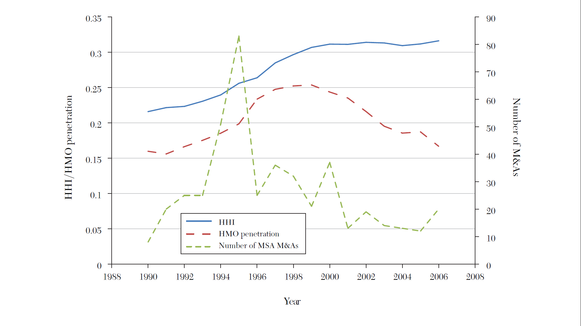
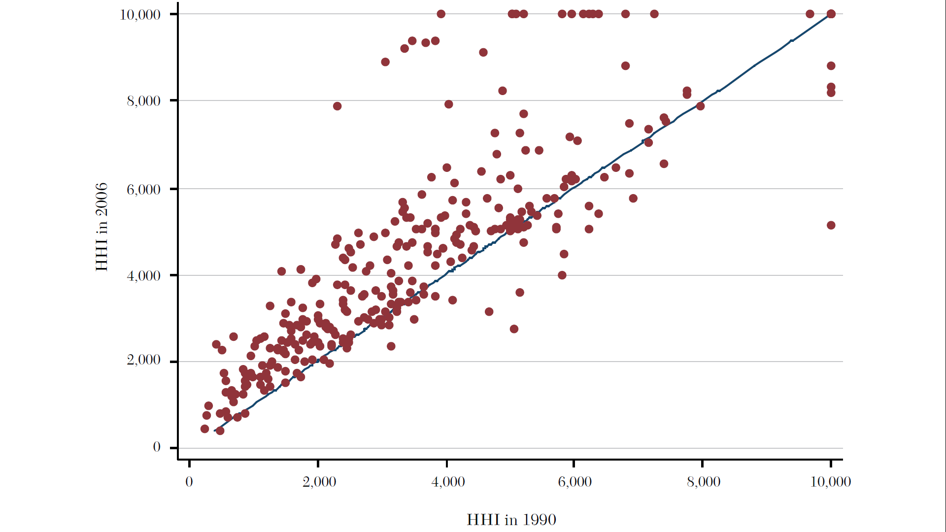
Source: Gaynor, Ho, and Town (2015). The Industrial Organization of Health Care Markets. Journal of Economic Literature.
Hospital concentration over time
- More data and interactive report from the Health Care Cost Institute.
- Presentation from the National Institute for Health Care Management
Why?
Historical perception of hospital competition as “wasteful” and assumption that more capacity means more (unnecessary) care:
- Limit public spending by limiting competition
- Prevalence of certificate of need (CON) laws
Effects of reduced competition
- Higher prices
- Lower quality, 2020 NEJM Paper
- Maybe lower costs (but not passed on to lower prices)
Effects for both “in-market” and “out-of-market” mergers
Measuring Competition
Importance of the market
Every analysis of competition requires some definition of the market. This is complicated in healthcare for several reasons:
- Hospital markets more local than insurance markets
- Hospitals are multi-product firms
- Geographic market may differ by procedure
- Insurance networks limit choice within a geographic market
Given a market
Once we have a measure of the market, we’d like to have a quick and easy way to assess competitiveness:
- HHI
- WTP
HHI
- Basic Cournot framework: \[\pi_{i} = P(q) q_{i} - C_{i}(q_{i})\]
- First order condition: \[P'(q) q_{i} + P(q) - C_{i}'(q) = 0\]
HHI
- Rewriting yields: \[\frac{P(q) - C_{i}'(q_{i})}{P(q)} = \frac{q_{i}}{q} \times \frac{-P'(q)q}{P(q)}=\frac{\alpha_{i}}{\eta}\]
- Constant marginal costs: \[\frac{p - c_{i}}{p} = \frac{\alpha_{i}}{\eta}\]
HHI
- In equilibrium, \[\sum_{i}\pi_{i} = \sum_{i}(p - c_{i}) q_{i} = \sum_{i}(p-c_{i})\alpha_{i} q\]
- Two equivalent expressions
- \(\sum_{i} \pi_{i} = \left(p - \sum_{i} \alpha_{i} c_{i} \right)q\) and
- \(\sum_{i} \pi_{i} = \frac{pq}{\eta} \sum_{i} \alpha_{i}^{2}\) after substituting \(p - c_{i} = \alpha_{i} \frac{p}{\eta}\).
HHI
- Equating these two expressions yields:\[\frac{p - \sum_{i} \alpha_{i} c_{i}}{q} = \frac{\sum_{i} \alpha_{i}^{2}}{\eta} = \frac{HHI}{\eta}\]
- Takeaway: In linear Cournot model with constant marginal costs and homogeneous products, the markup (a common measure of market power) is proportional to the HHI.
WTP
- Alternative measure from Capps et al. (2003)
- Not healthcare specific…option demand market where indermediary sells a “network” of products to consumers, and consumers are uncertain about final products they will need
- Key: consumers agree to ex ante restrict their choice set before they know what services are needed
- Derivation works backward…
WTP
Step 1. Derive ex post utility.
\[\begin{align*} U_{ij} &= \alpha R_{j} + H_{j}'\Gamma X_{i} + \tau_{1} T_{ij} + \tau_{2} T_{ij} X_{i} + \tau_{3} T_{ij} R_{j} - \gamma(Y_{i},Z_{i}) P_{j}(Z_{i}) + \varepsilon_{ij} \\ &= U(H_{j},X_{i},\lambda_{i}) - \gamma(X_{i})P_{j}(Z_{i}) + \varepsilon_{ij}, \end{align*}\]
which yields choice probabilities, \[s_{ij} = s_{j}(G,X_{i},\lambda_{i}) = \frac{\text{exp}(U(H_{j},X_{i},\lambda_{i}))}{\sum_{g\in G}\text{exp}(U(H_{g},X_{i},\lambda_{i}))}.\]
WTP
Step 2. Derive utility from access to network, \(G\), with \(U(H_{g},X_{i},\lambda_{i})\) taken as given.
The patient’s expected maximum utility across all hospitals is, \[V(G,X_{i},\lambda_{i}) = \text{E} \left[\max_{g\in G} U(H_{g},X_{i},\lambda_{i}) + \varepsilon_{g} \right] = \text{ln} \left[\sum_{g\in G} \text{exp} (U(H_{g},X_{i},\lambda_{i})) \right].\]
WTP
Contribution of hospital \(j\) is then:
\[\begin{align*} \triangle V_{j}(G,X_{i},\lambda_{i}) &= V(G,X_{i},\lambda_{i}) - V(G_{-j},X_{i},\lambda_{i}) \\ &= \text{ln} \left[ \left(\sum_{k\in G_{-j}} \frac{ \text{exp} (U(H_{k},X_{i},\lambda_{i})) }{\sum_{g\in G} \text{exp} (U(H_{g},X_{i},\lambda_{i})) }\right)^{-1} \right] \\ &= \text{ln} \left[ \left(\sum_{k\in G_{-j}} s_{k}(G,X_{i},\lambda_{i})\right)^{-1} \right] \\ &= \text{ln} \left[ \left( 1- s_{j}(G,X_{i},\lambda_{i})\right)^{-1} \right]. \end{align*}\]
WTP
Translate into dollar values by weighting by the marginal utility of price \[\triangle \tilde{W}_{j} = \frac{\triangle V_{j}}{\gamma (X_{i})}.\]
WTP
Step 3. Estimate ex ante WTP to include hospital \(j\) in patient’s network. (i.e., integrate over all possible health conditions)
\[W_{ij}(G,Y_{i},\lambda_{i}) = \int_{Z} \frac{\delta V_{j}(G,X_{i},\lambda_{i})}{\gamma (X_{i})} f(Z_{i}|Y_{i},\lambda_{i}) dZ_{i}.\]
Further integrating over all patients, \((Y_{i},\lambda_{i})\), yields \[WTP_{j} = N \int_{\lambda} \int_{Z} \int_{Y} \frac{1}{\gamma (X_{i})} \text{ln}\left[\frac{1}{1-s_{j}(G,X_{i},\lambda_{i})} \right]f(Y_{i},Z_{i},\lambda_{i})dY_{i} dZ_{i} d\lambda_{i}.\]
WTP in Practice
Simplify by calculating WTP for each “micro-market” (e.g., health condition) and taking sum:
\[WTP_{j} = - \sum_{m} N_{m} \text{ln}(1 - s_{mj})\]